Used-car price modeling

A comparison of regression methods for estimating used-car listing prices.

Held-out performance from our analysis. Adding categorical features helped much more than regularization. View full size (new tab): Bar charts comparing test R-squared and RMSE for five used-car regression models

What makes a listing expensive?

Our team compared used-car listing prices using numerical features and categorical information about the vehicle. The project started with ordinary least squares, then asked whether ridge regression, lasso, or a lower-dimensional PCA representation could improve the model. Listing prices are asking prices; they do not tell us what a buyer ultimately paid.

Building the linear model

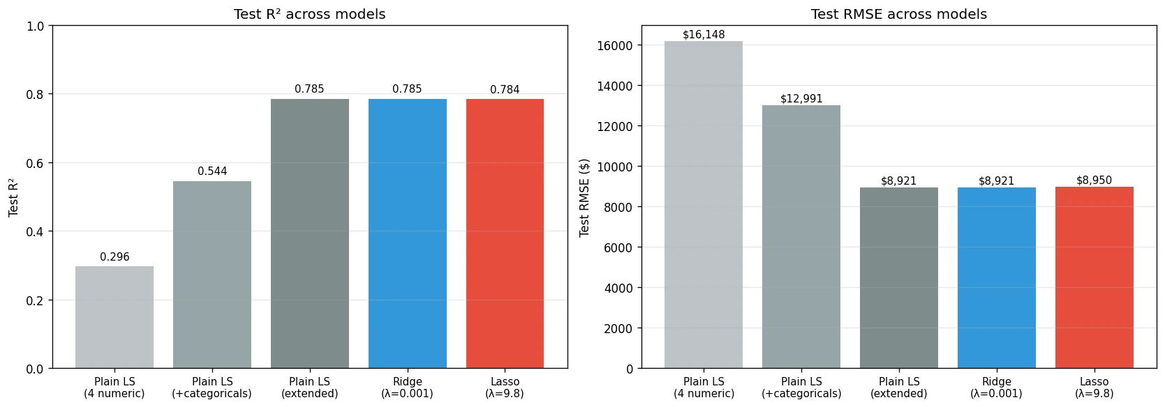
We derived least squares as an orthogonal projection and compared progressively richer feature sets. The four-numeric-feature baseline reached a test R² of 0.296. With the extended feature set, that rose to 0.785 and the RMSE fell from about $16,148 to $8,921. The extra vehicle information accounted for most of the improvement.

When regularization helped

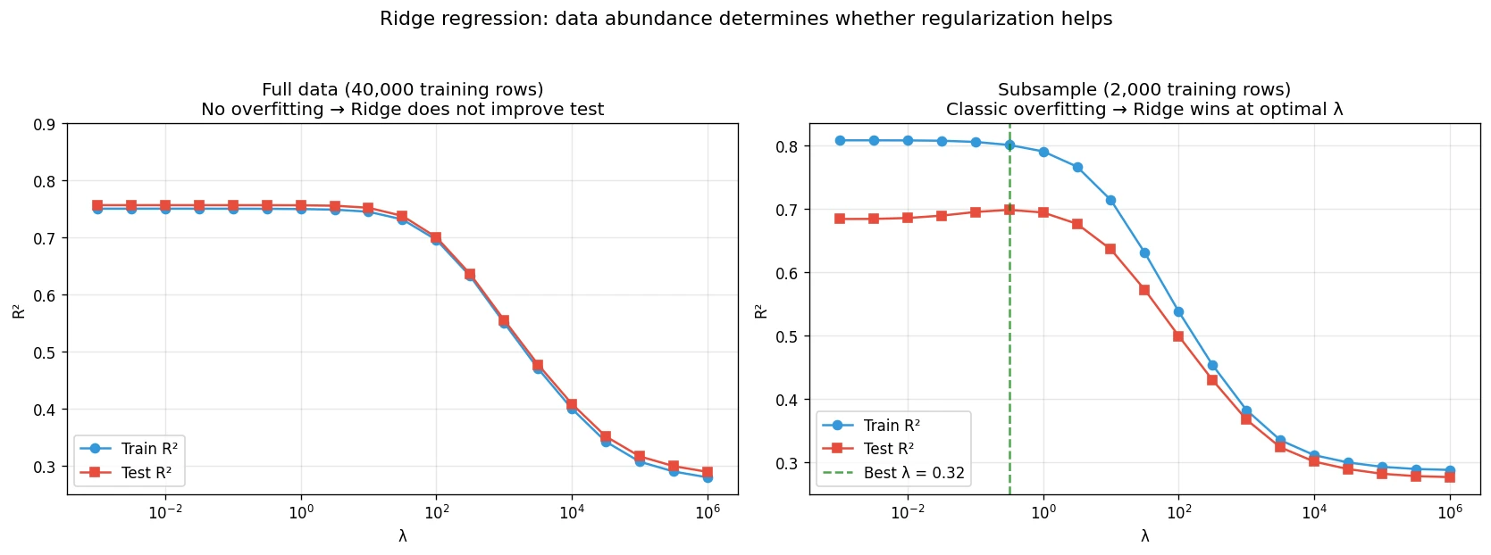
Ridge regression adds an L2 penalty to reduce large coefficients. On the full training sample, its best result was almost identical to ordinary least squares. The smaller-sample experiment made the tradeoff clearer: a modest penalty helped control the gap between training and test performance, while a large penalty underfit both.

The ridge sweep compares the full training sample with a 2,000-row subsample. View full size (new tab): Training and test R-squared versus ridge penalty for full and smaller training samples

Which features survived?

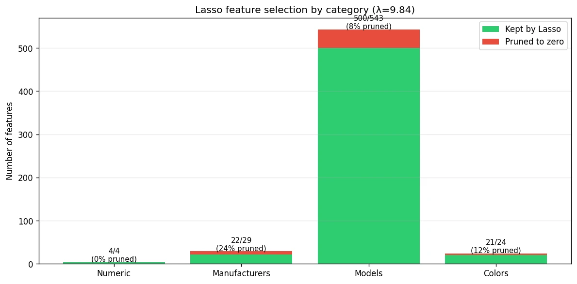
Lasso uses an L1 penalty, so some coefficients become exactly zero. The selected model kept 552 of 606 input features and reached a test R² of 0.784. It removed some manufacturer, model, and color indicators, but useful price information remained spread across many features.

Lasso retained all four numeric features and most categorical indicators. View full size (new tab): Stacked bars showing features kept and pruned by lasso across numeric, manufacturer, model, and color groups

Reducing dimensions

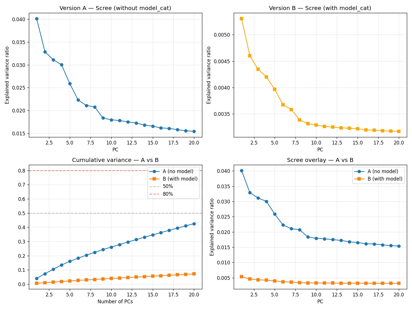
PCA let us examine how quickly a few directions capture variation in the feature matrix. The scree plots compare models with and without vehicle-model indicators. The cumulative curves helped explain why a very small set of components would discard information in the richer representation.

Principal components for the feature sets with and without model indicators. View full size (new tab): Scree plots and cumulative explained variance for two versions of the car feature matrix